Chronic obstructive pulmonary disease (COPD) is generally a slowly progressive airway disease that produces a decline in lung function that is not fully reversible. According to the World Bank/World Health Organization, COPD is expected to rise to the 5th ranked burden of disease by the year 2020.¹ COPD is most frequent in blue collar workers where tobacco smoking, occupational exposure, and socioeconomic status all contribute to the increased risk of the disease.² Thus, prevention of the development of COPD is an important public health issue worldwide and workplace screening may help in the prevention. The spirometry tests of forced vital capacity (FVC) and forced expiratory volume in one second (FEV1) are the recommended tests for the diagnosis of COPD.^1,3 Of the spirometry tests, the FEV1 is the most reproducible and best suited for measuring changes in lung function over time.⁴ Longitudinal FEV1 data allow us to study the rate of change in lung function, and to identify individuals and groups with an increased decline in lung function for an early intervention.^5–9 Potentially, workplace based spirometry monitoring can provide a valuable tool for an early recognition of excessive rate of lung function decline in an individual, that may reflect development of chronic lung diseases caused by occupational or environmental exposures, including smoking. However, the efficacy of the decision making based on longitudinal spirometry data in workplace monitoring programmes depends critically on the precision of the available longitudinal data—that is, the magnitude of within-person variation.¹⁰

The American Thoracic Society (ATS) provides guidelines for spirometry quality control that help to decrease measurement errors within single test sessions.¹¹ There is still a need, however, for statistical monitoring of precision when collecting longitudinal measurements over several years.¹² Such monitoring would enable one to investigate and reduce extraneous sources of random variation shortly after these arise, and, at the same time, attach a measure of precision to the data on which the decision making is being done.

In longitudinal spirometric data, precision is determined primarily by the magnitude of the within-person variation in lung function.^13–15 The sources of the within-person variation can be broadly categorised as those arising from measurement procedures (for example, spirometer, subject, or technician procedural errors) and those arising from the within-person fluctuation in lung function around its “true” value.^14,15 Figure 1 illustrates longitudinal FEV1 values for three individuals in our study who had different levels of within-person standard deviation S_ri around their individual linear regression lines. When examining an individual person’s longitudinal data it is important to know the magnitude of the average within-person variation for the group. This statistic provides an indication of the overall precision of measurements in a specific monitoring programme and influences how to interpret yearly declines that may be excessive.

The objective of the present study is to describe and investigate two statistical methods—a pairwise estimate of within-person standard deviation s_p and the reliability coefficient G—for use in the monitoring of the magnitude of the average within-person standard deviation σ_w (that is, data precision) in longitudinal FEV1 measurements in a group.^12,16,17 Using data from 11 large spirometry screening programmes,¹⁸ we investigated the ability of the two statistics to predict the magnitude of the within-person standard deviation as estimated from all longitudinal measurements. Secondly, we also investigated how the precision of longitudinal FEV1 measurements impacts on the detection of the “true” excess rates of decline in an individual.

MATERIALS AND METHODS

Lung function monitoring programmes

In our study we used data from spirometry monitoring programmes implemented in 11 industrial plants during the period 1987–2001. Pulmonary function testing and a medical, smoking, and occupational questionnaire were administered by trained personnel (NIOSH Spirometry Course # 002 presented by one of the investigators, HWG), using a computer system designed to collect such data from remote facilities.¹⁸ This system employs a computer with a resident questionnaire and an online, 8 l, dry rolling seal volumetric spirometer. Validation of the accuracy of this spirometric system¹⁹ has shown that it complied with ATS spirometric test criteria.^20,21 A 3 l calibrating syringe was used for daily calibration. Testing was conducted in the standing position with nose clips, and height was measured without shoes. Spirometric test results were taken from at least three acceptable tests with good initial effort (extrapolated volume less than 5% of the FVC, with distinct superimposable, forced expiratory flow volume curves),²² good continued effort for at least seven seconds, and repeatable FEV1 and FVC values within 5% or 100 ml. The final database included the largest FEV1 and FVC, and FEV1/FVC computed from the largest values. Quality assurance of the spirometric tests was done by one of the investigators (HWG).

Per cent predicted lung function values were computed for all study subjects using race and sex specific (White and African-American) prediction equations which included height, age, and age². These equations were developed from blue collar never-smokers who denied occupational inhalant exposures, and who were tested on the same type of equipment as in the present study.²³

The individual worker’s participation in the monitoring programme in each plant was voluntary and began either when the monitoring programme started or when a worker became employed at that facility, and stopped either on cessation of monitoring or on cessation of employment. For the purpose of our analysis, time of follow up was represented either by the calendar year of lung function testing (1987–2001) or by the years of follow up. The data from workers who were age 20 years or older were used to estimate the yearly within-person variation, the coefficient G, and the longitudinal within-person variation estimated by the mixed effects model. The data from workers who were 25 years and older and who had at least three measurements with five or more years of follow up were used to estimate the longitudinal within-person variation by the linear regression analysis.

Statistical methods

Outline

We “monitored” the precision of FEV1 measurements on a yearly basis within a period 1987–2001 separately in each of the 11 plants. We used two statistics to monitor the average within-person variation in each plant: (1) the pairwise estimate of within-person standard deviation s_p, and (2) the reliability coefficient G. To evaluate usefulness of these estimates, we correlated the plant specific mean values s̄_p and Ḡ (calculated as the averages of the yearly values of s_p and G, respectively), to the average plant specific within-person standard deviation estimated from all longitudinal data by the linear regression model (s_r) or the mixed model (s_m). Finally, we showed how the plant specific within-person variation impacts on the ability to detect significant excess rates of decline in FEV1 in an individual. The following four subsections provide further details on the statistical methods.

Estimation of the group within-person variation from pairwise measurements

Consecutive measurements of FEV1 (M_a and M_b), taken within a short duration from each other on a group of workers can be used to assess the group average within-person variability as follows.

1. The pairwise estimate of the within-person standard deviation can be estimated from the difference between the two measurements M_a and M_b as

where the summation in a specific plant is over n subjects.

2. The coefficient of reliability G can be estimated from the following formula:

G = S_b²/(S_b²+S_w²)

where S_b² is the between-subject variance and S_w² is the within-person variance. For a given S_b², increasing S_w² leads to a lower G value—that is, a lower data precision. A simple method of estimation of the coefficient G is to calculate the Pearson correlation coefficient r_MaMb on the consecutive measurements M_a and M_b.^12,16,17 To remove variation due to systematic population effects such as age, height, sex, or race, the correlation should be done on the percent predicted values. (Because an additional source of error can be introduced by errors in these covariates, these should be kept constant as much as possible.)

The interval between two measurements M_a and M_b should be sufficiently long to include all potential short term random effects, but short enough to avoid time related systematic changes—for example, those due to age. In the present analysis, year specific values of s_p and G were calculated by using two FEV₁ measurements repeated within 18 months; this period was chosen for practical reasons for yearly monitoring. We have established previously¹² and in our current study, that the value of the coefficient G does not change much when the period between two measurements is increased from 12 to 18 months. The reason for this is that the variability in the expected decline in FEV1 per year is much smaller than the random variation around the slope.¹³ The date of the first test determined the follow up year. This procedure gave us a sufficient number of tests per year while not noticeably affecting the yearly values of s_p and G when compared with a 12 month period. In the few cases where there were more than two repeated tests, only the first pair of tests per subject was used within the follow up year. Note that this strategy is appropriate for workplace monitoring programmes where annual measurements are available on all individuals or on a random sample of individuals.

Estimation of the within-person variation from all longitudinal data

The average plant-specific within-person standard deviation was estimated from all the longitudinal data using the following two methods:^24,25

1. Estimation by the two-stage method. In the first stage, we fitted the linear regression model, FEV1_i = β_0i+β_1i·time+ε_i, to each i-person’s vector of repeated FEV1 measurements and the time covariate (years of follow up). The individual within-person variance S_ri² was estimated by the regression MSE_i. In the second stage, we estimated the average plant-specific within-person standard deviation s_r as the square root of the mean S_ri² calculated across all subjects. (Because of the relatively short follow up time, we assumed that the longitudinal FEV₁ values were linearly related to time, with a constant variance.) We estimated the plant-specific s_r using individuals with five or more years of follow up.²⁶

2. Estimation by the mixed effects model. The mixed model is represented by the equation Y_i = X_iβ+Z_ib_i+ε_i, where, for the i-person, Y_i represents the vector of repeated FEV1 measurements, X_i is the matrix of fixed (population) covariates, β is the vector of unknown regression coefficients for the population covariates, Z_i is the matrix of random subject-specific time covariates, and b_i is the vector of unknown subject-specific estimates of random effects (that is, the intercept and slope for time). We fitted the above mixed model to each plant-specific set of data to estimate the plant-specific within-person standard deviation s_m from the residual variance.^24,25 Individuals with at least one follow up measurement were included in this analysis (n = 6440). The fixed effects included in our model were age, height, sex, race, wheezing, smoking status, and time variant pack years (that is, pack years cumulated with increasing years of follow up).

Impact of group data precision on identifying excessive decline in FEV1

To illustrate the effect of the group data precision on our ability to identify an excess rate of decline in FEV1 in an individual, we used as an example two people, both having an FEV1 of 4 l at 34 years of age and an expected “normal” rate of decline of 30 ml/year,²⁷ but one being from a plant where data are collected with high precision (PLANT-HP) and the other from a plant where data are collected with low precision (PLANT-LP).

Firstly, we derived the approximate longitudinal one sided 95% confidence limit for an expected decline, b, over a specific duration, D (years). This limit is given by D×[b + 1.645×SE(b)]. Subtracting this limit from the initial FEV1 measurement gives the lower limit of normal for the FEV1 measurement (LLNR), as derived using the formula:^28,29

LLNR =  initial FEV1- D×[b + 1.645×SE(b)]

where D is duration of follow up in years starting at D = 1 at 35 years of age and incrementing by one at each year, and the term [b + 1.645×SE(b)] determines the maximal regression slope of decline for an expected FEV₁ decline (that is, 30 ml/year). The standard error of the slope b, SE(b), is derived from the formula derived by Schlesselman:³⁰

where P is the number of tests done during D years of follow up. Schlesselman’s method of estimation was also applied previously to estimate sample size for longitudinal spirometry studies.^13,31,32

The value of σ_w in the SE(b) formula was estimated by the average within-person standard deviation s_r for plants in our study that had the highest precision PLANT-HP and lowest precision PLANT-LP, respectively.³⁰ Because the estimate of within-person variation σ_w is derived from a large number of subjects, we assume the normal standard deviate for a one sided limit when p value is 5% to be Z_α = 1.645.

The estimate of LLNR was based on SE(b) derived for a specific number of tests P done during the D years of follow up. Similarly, [b + 1.645×SE(b)] provides a limit of normal rate of decline given the parameters σ_w, D, P. Any individuals having observed declines below or rates of decline above these two types of limits would be detected as having an excess decline. Hence in subsequent discussion we refer to these two criteria as the detectable excess decline and the detectable excess rate of decline.

Variability in longitudinal data

To investigate how well the estimated LLNR agree with the observed data, we also show variability in the rate of change in FEV1 observed within one year, summed over all individuals and years, for the plants with the highest and lowest data precision. The rate of change in FEV₁ (l/year) was calculated as a difference between two repeated measurements done within 12 months of each other.

RESULTS

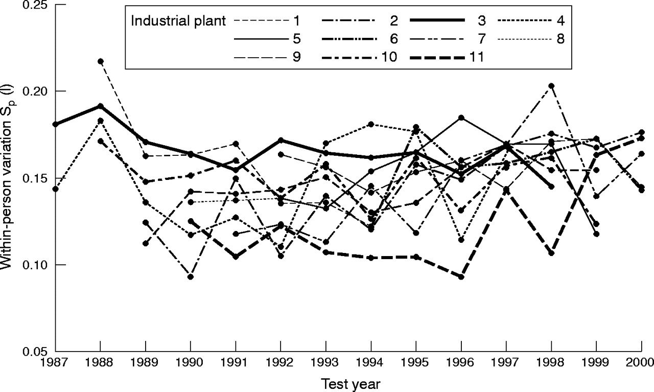
Table 1 gives, for the 11 plants, the number of workers who participated in the monitoring by follow up years. Table 1 also shows the number of workers who had at least three measurements over five or more years of follow up after 25 years of age (n = 3130). Figure 2 shows the plant-specific yearly values of within-person standard deviation s_p; the plants with consistently high and low values of s_p are indicated by thicker lines.

Table 2 shows the plant-specific values of s̄_p and Ḡ calculated as means of the yearly values, and their coefficients of variation (CV). Table 2 also shows plant-specific within-person variations s_r and s_m estimated from longitudinal data using the two-stage method and the mixed model. The correlations between the variables are shown at the bottom of the table.

Table 2 shows that, on the basis of the values of s̄_p, plants 11 and 3 have the highest and lowest data precision, respectively. These two plants are used to represent PLANT-HP and PLANT-LP, respectively. For PLANT-HP, s̄_p = 0.122 l, Ḡ = 0.954, s_r = 0.130 l, and s_m  = 0.124 l. For PLANT-LP, s̄_p = 0.166 l, Ḡ = 0.898, s_r  = 0.177 l, and s_m  = 0.173 l.

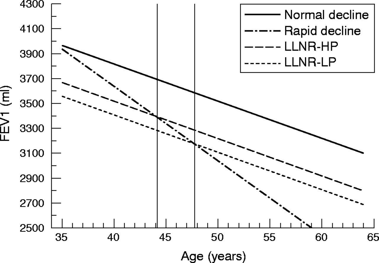
Figure 3 shows the longitudinal lower limits of normal LLNR for the “normal” decliners from PLANT-HP (LLNR–HP) and PLANT-LP (LLNR-LP), respectively. The LLNR were estimated for P = 2, that is, for two tests done at the start of monitoring at age 34 and at various specific ages thereafter. Figure 3 also shows a predicted line for a person with a rapid decline of 60 ml/year and the ages at which a rapid decliner’s predicted line crosses the longitudinal LLNR-HP or LLNR-LP.

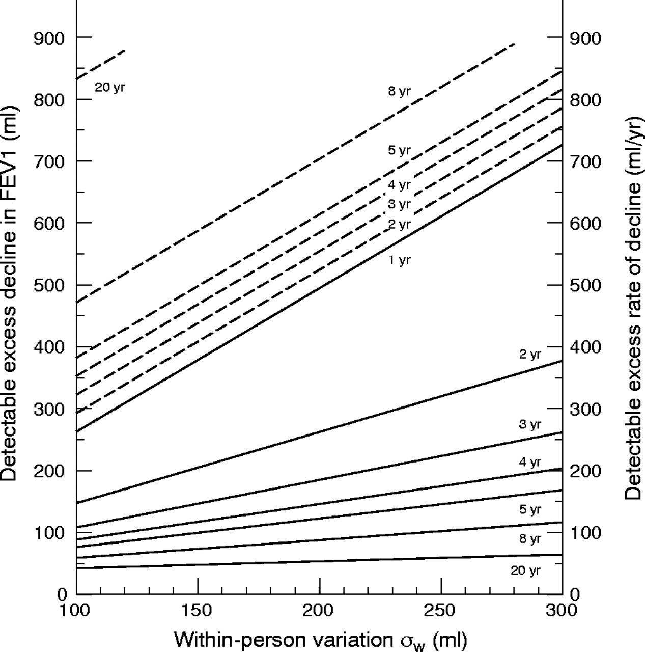
Figure 4 shows on the left vertical axis the detectable excess decline in FEV1 (ml) and on the right vertical axis the detectable excess rate of decline in FEV1 (ml/year) defined by the limit of normal for an individual person after D = 1, 2, 3, 4, 5, 8, 20 years of follow up, for a known magnitude of the within-person variation σ_w, based on two measurements. The solid line for one year of follow up represents the detectable excess decline and also the detectable rate of decline. According to this line, the detectable excess decline is ≈ 260 ml when σ_w  = 100, ≈ 375 ml when σ_w  = 150, and ≈ 500 ml when σ_w  = 200.

The right vertical axis and the solid lines of the figure show how the detectable excess rate of decline becomes smaller as the duration of follow up increases (the procedure becomes more sensitive). For example, with a data precision σ_w  = 150, the detectable excess rate of decline decreases with an increasing duration of follow up, D = 1, 2, 3, 4, 5, 8, 20, as 375 ml/year, 200 ml/year, 150 ml/year, 120 ml/year, 100 ml/year, 80 ml/year, and 50 ml/year, respectively. Note that one needs data precision of σ_w  = 130 to detect a “true” slope of 90 ml/year after five years of follow up; this slope was recommended by the American College of Occupational and Environmental Medicine (ACOEM) to be considered as significant loss of lung function.^33,34

To establish how well the estimated excess decline for one year agrees with observed data, we calculated the percentile statistics for the observed yearly changes in FEV1 (calculated across all subjects and all years of follow up) for plant 11 and plant 3. These yearly changes represent the observed yearly fluctuation in FEV1. For plant 11, 95% of the negative changes (that is, the 5th percentile) were within −342 ml per year. For plant 3, 95% of the declines were within −433 ml per year. When we calculated the observed yearly changes in FEV₁ for groups of plants with s_r ≈ 0.15 (plants 5, 18, 22) and plants with s_r ≈ 0.16 (plants 8, 9, 13, 15) (table 2), the 5th percentiles were −0.394 ml and −0.389 ml, respectively. These results agree approximately with our estimates from figure 4, for one year of follow up.

DISCUSSION

Decision making based on imprecise longitudinal spirometry is likely to be ineffective and can be even counterproductive. A major task in longitudinal screening programmes and studies is to maintain a continued low level of within-person variation. This ensures that an individual’s rate of change in lung function is estimated reliably. Due to the increased accuracy of commercially available spirometers, the random measurement error due to an instrument error (calibration procedures, malfunction, and so on) can be minimised, but other sources of the within-person variation still remain an issue.^15,22

The results from our study show that by monitoring the precision of the longitudinal data using the within-person standard deviation s_p based on two repeated measurements or the G statistic, one can predict the magnitude of the within-person variation estimated from longitudinal data with five or more years of follow up. The plant-specific within-person variation s̄_p correlated more strongly with the longitudinal estimate s_r than the plant-specific coefficient Ḡ, and thus it may be more suitable for monitoring of data precision especially in a smaller sample. However, the values of s̄_p were systematically lower than those of the longitudinal s_r or s_m, which may be because the shorter follow up does not include all potential errors that can occur during the longer follow up and also because of autocorrelation.³⁰

The advantage of the coefficient G is its simplicity of estimation. Our data suggest that the value of coefficient G estimated from per cent predicted FEV1 values should be maintained above 0.90 at minimum, but ideally above 0.95. Although the coefficient G is easy to calculate, it has some inherent limitations. Because G is determined by the magnitude of the between-person variance as well as the within-person variance, in smaller samples, significant fluctuations in G may arise from fluctuation in the between-person variation, and it may be better to employ the within-person standard deviation s_p estimate. Based on our observations, the coefficient G based on per cent predicted values and a minimum sample size over 100 reflects changes in the within-person variability almost as well as the s_p statistic.

The 11 plants that we investigated used standardised spirometry methods based on ATS recommendations. The range of plant-specific s_r based on slopes with at least five years of follow up was 0.130–0.179 l (see table 2, two-stage). These values are comparable to previously published values for large monitoring programmes (0.114–0.160 l).¹³ Because the values of the within-person variation did not change substantially after we adjusted for age, height, symptoms of wheezing, and time variant smoking in the mixed model, we suspected that differences in measurement procedures, especially variability in technicians may have been the main sources of the within-person variation. Based on incomplete technician records, the testing in plant 11 was done by two technicians, whereas in plant 3 at least six technicians performed the testing. We also cannot exclude the possibility that occupational exposure increased the within-person variation in some plants.

Monitoring and maintaining data precision is important. Based on theoretical considerations, we show that the degree of precision in longitudinal FEV1 measurements affects the ability to detect abnormal decline in individuals. Figure 3 shows that the LLNR, based on the group average within-person variation, is higher for a person from PLANT-HP than for a person from PLANT-LP. The increased precision in longitudinal measurements affects the ages when the rapid decliner of 60 ml/year is crossing the LLNRs. For the LLNR-HP (s_r = 0.130 l), the intersection is at ≈ 44 years of age. For the LLNR-LP (s_r = 0.177 l), the intersection is at ≈ 48 years of age. Thus, the precision of the longitudinal data can affect the age at which we can identify a “true” rapid decliner. However, if we used the LLNR-HP for a decision-making in PLANT-LP, we could identify “false” rapid decliners because the random variation in FEV1 in PLANT-LP is higher than in PLANT-HP.

A recent study suggests that a yearly decline of 8% or 330 ml should not be considered normal in healthy working males tested according to ATS standards.³⁵ Similarly, in the Lung Health Study, 95% of the yearly differences in FEV1 were within 320 ml for men with early COPD.³⁶ Figure 4 shows that for the duration of follow up D = 1 and number of tests P = 2, in 95% of individuals the yearly decline in FEV1 would be within ≈ 330 ml for σ_w of 130 ml.

Figure 4 illustrates how the size of the within-person standard deviation σ_w can impact the detection of excess decline in FEV1 (dashed line) and excess rate of decline (solid line), for a given duration of follow up D and two repeated measurements. It takes longer in an imprecise monitoring programme to identify a “true” excessive rate of decline in FEV1. For example, it takes five years to identify an excess rate of decline of 90 ml/year when σ_w  = 130 ml and eight years when σ_w  = 210 ml. Conversely, after five years of follow up the detectable excess rate of decline increases with increasing value of σ_w as follows: for σ_w  = 100 it is 75 ml/year, for σ_w  = 130 it is 90 ml/year, for σ_w  = 150 it is 100 ml/year, for σ_w  = 250 it is 150 ml/year, and for σ_w  = 300 it is 170 ml/year. The 5th percentiles for the observed yearly changes in FEV1 found for our plants 3 (−0.342) and plant 11 (−0.433) agreed with the estimated data for one year of follow up in figure 4.

For example, in figure 1 one may not consider the decline of 400 ml from the first to the second FEV1 observation for person B to be abnormal if the value of s̄_p for the monitoring programme is 200 ml. However, one should try to identify extraneous sources of within-person variation and decrease s_p. If, on the other hand, s̄_p is ≈ 100 ml, then one should consider the decline of 400 ml excessive and take appropriate action.

These results show that a measure of data precision needs to be attached to the longitudinal data on which decision making is being made even if the subjects are tested according to the ATS recommendations. One can also increase precision of the estimated slopes by increasing the number of observations for an individual person whose measurements fall bellow the longitudinal lower limits of normal. An abnormal decline based on a predicted slope estimated over five or more years of follow up could then trigger more definite intervention measures.

In conclusion, the results demonstrate that there is a need for monitoring of data precision in spirometry monitoring programmes performed by technicians trained in ATS standards. For a little additional cost, the gain in the precision of the estimates on which decision making is made could be invaluable as it would allow identification of rapid decliners at an earlier age and prevent development of airflow obstruction.