Article Text

Abstract
Study objectives: This study examines the influence of individual and neighbourhood socioeconomic status (SES) on mortality among black, Mexican-American, and white women and men in the US. The authors had three study objectives. Firstly, they examined mortality rates by both individual level SES (measured by income, education, and occupational/employment status) and neighbourhood level SES (index of neighbourhood income/wealth, educational attainment, occupational status, and employment status). Secondly, they examined whether neighbourhood SES was associated with mortality after controlling for individual SES. Thirdly, they calculated the population attributable risk to estimate the reduction in mortality rates if all women and men lived in the highest SES neighbourhoods.
Design: National Health Interview Survey (1987–1994), linked with 1990 census tract (neighbourhood proxy) and mortality data through 1997.
Setting/participants: Nationally representative sample of 59 935 black, 19 201 Mexican-American, and 344 432 white men and women (six gender and racial/ethnic groups), aged 25–64 at interview.
Main results: Mortality rates for all six gender and racial/ethnic groups were two to four times higher for those with the lowest incomes (lowest quartile) who lived in the lowest SES neighbourhoods (lowest tertile) compared with those with the highest incomes who lived in the highest SES neighbourhoods. For the six groups, the age adjusted mortality risk associated with living in the lowest SES neighbourhoods ranged from 1.43 to 1.61. The mortality risk decreased but remained significant (p values <.05) after adjusting for each of the three individual measures of SES, with the exception of Mexican-American women. Furthermore, the mortality risk associated with living in the lowest SES neighbourhoods remained significant after simultaneously adjusting for all three individual measures of SES for white men (p<0.001) and white women (p<0.05). Deaths would hypothetically be reduced by about 20% for each subgroup if everyone had the same death rates as those living in the highest SES neighbourhoods (highest tertile).
Conclusions: Living in a low SES neighbourhood confers additional mortality risk beyond individual SES.
- ethnic goups
- mortality
- residence characteristics
- socioeconomic factors
Statistics from Altmetric.com
The importance of neighbourhoods in our life cycles has long been observed. Over 30 years ago Rossi noted that our neighbourhoods provide the medical facilities in which we are born, the schools in which we are taught, the housing in which we live, the social milieu in which we set up our households, the factories and businesses where we find work, and finally the cemeteries where we are buried.1 While factors beyond our neighbourhoods also affect our lives, the local community plays an important part in shaping our daily experiences and is the setting in which many social, economic, and political policies have an impact.2
It is logical that the neighbourhood socioeconomic environment plays an important part in our health. This may occur, in part, via access to goods and services (for example, education and employment opportunities; price, availability, and quality of goods and services), norms and values, and the physical environment (for example, air and water quality). Despite the fact that neighbourhoods, as well as people, are stratified along socioeconomic lines, surprisingly few studies have focused on the role of the neighbourhood environment in shaping the health of its residents. Studies have more commonly focused on how individual socioeconomic characteristics influence health.3–8 However, there is a growing consensus that socioeconomic characteristics of neighbourhoods may influence both the socioeconomic status (SES) and health of its residents.
Findings from historical and contemporary epidemiological studies that have examined individual SES and mortality have consistently shown that women and men with low SES, regardless of how it is measured, have higher death rates than their higher SES counterparts.8–11 Recent studies have examined neighbourhood SES and mortality, focusing on the broader social context within which health related behaviours, decisions, and events occur. Findings from these studies indicate that neighbourhood SES is associated with individual level mortality, independent of individual SES.9,12–21 This suggests that characteristics of places represent more than the aggregation of characteristics of their residents. The magnitude of the neighbourhood effects in these studies has generally been modest. However, it is difficult to determine the extent to which individual level SES is on the pathway between neighbourhood SES and mortality (that is, is a mediator rather than a confounder) so that the effect of neighbourhood SES on mortality could be underestimated after adjusting for individual SES.
This study extends the existing literature on neighbourhood SES and individual level mortality, while considering the effects of individual SES. We used a nationally representative sample that includes the three largest racial/ethnic groups of women and men in the US. We stratified by racial/ethnic group because we hypothesised that neighbourhood effects could potentially vary across groups given that patterns of residential segregation are closely related to socioeconomic segregation. We had three study objectives. Firstly, we examined mortality rates by both individual level SES (measured by income, education, and occupational/employment status) and neighbourhood level SES (index of neighbourhood income/wealth, educational attainment, occupational status, and employment status). Secondly, we examined whether neighbourhood SES was associated with mortality after controlling for individual SES. Thirdly, we calculated the population attributable risk to estimate the reduction in mortality rates (that is, number of lives saved) if all women and men lived in the highest SES neighbourhoods.
METHODS
Data sources
We used data from the National Health Interview Survey (NHIS) from 1987–1994. We linked these data to the 1990 US. Census for neighbourhood SES and to the National Health Interview Survey/Multiple Cause of Death Public Use Data file (NHIS/NDI) for mortality through 1997. We included data for black, Mexican-American, and white women and men, aged 25–64 at interview. This age group was selected to ensure that most people had completed their education and because previous research has found that SES differences in health are greater for young and middle aged adults compared with the elderly population.10,22,23 The NHIS data were collected through a continuing survey of US households in a multistage design where a probability sample of the civilian population is drawn each week.24,25
The NHIS/NDI file was produced by the National Center for Health Statistics by matching characteristics from the NHIS and the National Death Index (NDI), allowing for a follow up mortality link with survey data.26 The NDI was searched from the month and year of the NHIS interview to 31 December 1997, making the shortest follow up period one month and the longest follow up period 11 years. The final sample consisted of 59 935 black, 19 201 Mexican-American, and 344 432 white women and men (table 1).
Addresses of the respondents in each annual NHIS file have been geocoded to 1990 census geography, which was used to link characteristics of the respondents’ place of residence using census tract level data. Census tracts include about 4000 to 7000 people, have boundaries that represent comparatively homogeneous populations in terms of social and economic characteristics,27,28 and have been used extensively as proxy measures of neighbourhood environments. Only 5.4% of respondents were missing geographical identifiers and were not included in the analysis.
All research was approved by the appropriate ethics committee at Stanford University, School of Medicine and conforms to the principles of the Declaration of Helsinki.
Definition of variables
Individual level SES was defined by three measures: educational attainment, income-to-needs ratio (annual income per family member), and a combined measure of occupational and employment status. We operationalised educational attainment into categories based on achieved credentials (less than 9 years, 9–11 years, 12 years, more than 12 years). The income-to-needs ratio was calculated by dividing the midpoint of the categories for family income by family size as the resources available to a family size of one with $50 000 are very different than to a larger family size with the same income. The midpoint of family incomes above $50 000 (the highest cut off in the NHIS) was assigned a value of $75 000 (which was just below the average family income of $79 000 for families making over $50 000 according to the 1990 US census).29 We operationalised income into gender and racial/ethnic group specific empirical quartiles because previous research on the effects of income on health outcomes has shown non-linear effects30 and because categorising income allowed us to include an indicator variable for those with missing income data (see appendix). We operationalised occupational/employment status into four standard census based categories: not in the labour force (including retired persons, homemakers, students), unemployed, blue collar workers (service, farming/forestry/fishing, precision production/craft/repair, and operator/fabricator/laborer occupations), and white collar workers (managerial/professional specialty, and technical/sales/administrative support occupations). We excluded persons in the military and those with unknown occupations. Correlations among the three individual SES measures were 0.48 or below for the overall sample and for each racial/ethnic group.
To define neighbourhood level SES, we performed a principal components analysis using standardised values of five census tract variables to represent neighbourhood level educational attainment (percentage of persons 25 years and over without a high school degree), income (median family income), wealth (median housing value), occupational status (percentage blue collar workers), and employment status (percentage unemployed). The first component accounted for almost 60% of the variance. All five variables contributed about equally to the component; therefore, we calculated our neighbourhood SES index as the mean of the standardised values with equal weights. We compared the neighbourhood SES index to one based on centile ranks to examine whether outliers influenced the index and found that the two indices were highly correlated (0.96); therefore, we used the index based on the means of the standardised values in our analyses. We operationalised the neighbourhood SES index into gender specific and racial/ethnic group specific empirical tertiles (see appendix). Previous analyses have found this sample of census tracts to be nationally representative of all US census tracts in terms of socioeconomic characteristics.31
Race/ethnicity was self reported and included persons who identified themselves as either black (non-Hispanic), Mexican-American (Mexican-Mexicano, Mexican-American, Chicano), or white (non-Hispanic). Other racial/ethnic groups were excluded from the analysis because of small sample sizes.
Analytical approach
We calculated age adjusted, all cause mortality rates per 100 000 person years for the follow up period by dividing the number of deaths by the number of person years of follow up. Mortality rates are presented for women and men for the three racial/ethnic groups, stratified by individual and neighbourhood SES. Relative rates of mortality were obtained using Cox proportional hazards regression models. The final models were estimated with the summary neighbourhood SES index as well as with each component of the index and similar patterns were found. The population attributable risk (PAR) was calculated using the overall death rates compared with the rates for those living in the highest SES neighbourhoods, without regard to individual SES. Thus, the PAR represents the proportional reduction in mortality that would occur if everyone experienced the mortality rates of those living in the highest SES neighbourhoods.
As the NHIS is a complex multistage probability sample that yields clustered observations, we used SUDAAN (version 7.5.6, Research Triangle Institute, 2000) to account for the survey design effects and to produce valid variance estimates in our regression models.32 SUDAAN also alleviates difficulties with statistical inference introduced by multilevel research designs.33,34 Multilevel linear modelling techniques35,36 were not used in this analysis because, while the number of census tracts (or neighbourhoods) was large for each group, there were few adults sampled per tract (about two persons sampled per tract).37 Given that our data, in large measure, are not nested (that is, few sampled per tract) and that one person’s mortality is not likely to affect another person’s in the same tract (that is, low intercorrelation coefficient), we feel that this analytical approach is appropriate. Previous studies have used a similar analytical approach.12,14,15,33,38–41
RESULTS
Black and Mexican-American women and men lived in lower SES neighbourhoods compared with white women and men, as measured by our neighbourhood SES index. As illustrated in figure 1, there was little overlap in the middle tertile of the SES index when comparing the white population with black population and Mexican-Americans. The values within each tertile represent very different neighbourhood conditions. For example, neighbourhoods with a SES index value of 1 (the approximate upper value for the middle tertile of neighbourhood SES for the black population and Mexican-Americans) compared with 0 (the approximate upper value for the middle tertile of neighbourhood SES for the white population) had 40% more blue collar workers (60% v 43%), twice the proportion of residents without a high school degree (44% v 21%), two thirds the median family income value ($21 000 v $33 000), 40% lower housing values ($48 000 v 68,000), and 50% higher unemployment rates (6.1% v 4.1%). Because of these differences we stratified the analyses by race/ethnicity so that the results can be interpreted within each racial/ethnic group.
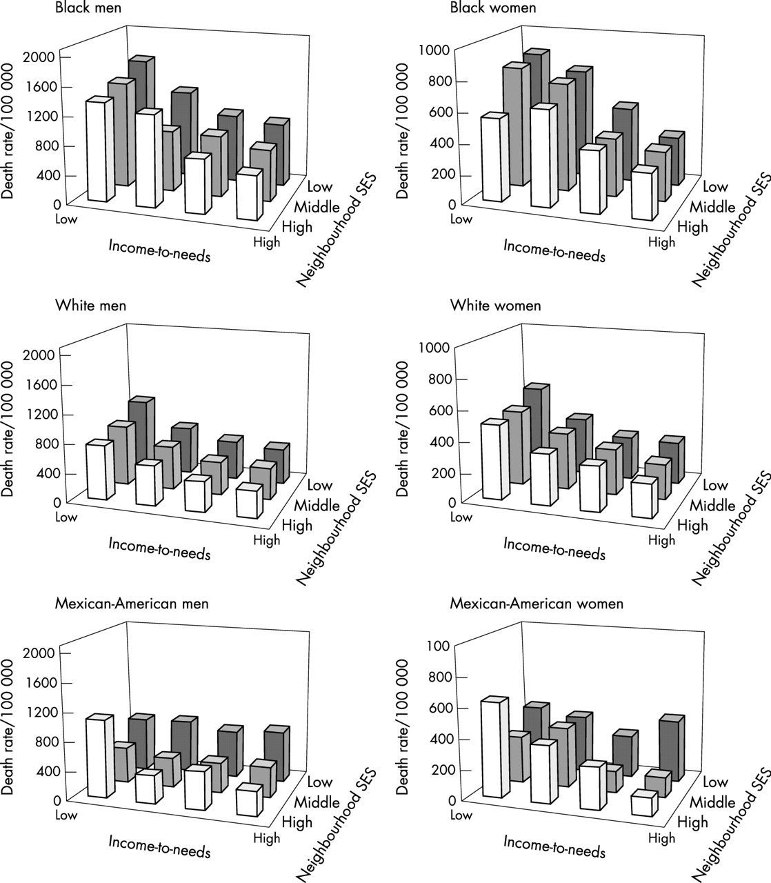
The age adjusted mortality rates per 100 000 person years by individual SES (in this case, income to needs ratio) and the neighbourhood SES index are shown in figure 2. For all comparisons, there was a more pronounced gradient between individual SES and mortality than for neighbourhood SES and mortality. Overall, mortality rates were higher for men than for women (note the different scales for the mortality rates), and were highest for black men and women. Death rates generally increased as neighbourhood SES decreased, with the exception of Mexican American men and women for whom the patterns were less consistent. One noticeable exception was that the highest death rates for Mexican-American women and men were for those with the lowest family incomes who lived in the highest SES neighbourhoods. Death rates for all six gender and racial/ethnic groups were two to four times higher for those with the lowest incomes (lowest quartile) who lived in the lowest SES neighbourhoods (lowest tertile) compared with those with the highest incomes who lived in the highest SES neighbourhoods. The relations between educational attainment and occupational/employment status with neighbourhood SES were less consistent (data not shown). This is possibly because of smaller sample sizes within certain categories (for example, number of unemployed).
To examine whether living in a low SES neighbourhood conferred additional mortality risk beyond individual SES, we calculated relative mortality ratios from age adjusted Cox proportional hazards models (tables 2 and 3). We estimated five models for each of the six groups. The independent variables were: age and neighbourhood SES (model 1); age, one of the individual SES variables (income to needs, educational attainment, or occupation/employment status) and neighbourhood SES (models 2–4); and age, all three individual SES variables, and neighbourhood SES (model 5). For the six groups, the age adjusted mortality risk associated with living in the lowest SES neighbourhoods ranged from 1.43 to 1.61 (a 43% to 61% increased risk) (model 1). The mortality risk decreased but remained significant (p values <0.05) after adjusting for each of the three individual measures of SES, with the exception of Mexican-American women (models 2–4). As an example, for white women, the 43% increased risk in mortality associated with living in a low SES neighbourhood decreased to 18% when adjusting for the income to needs ratio, to 22% when adjusting for educational attainment, and to 36% when adjusting for occupation/employment status. In model 5, living in a low SES neighbourhood was associated with an 11%–18% increase in the risk of mortality for white women and men respectively, which remained statistically significant after simultaneously adjusting for all three measures of individual SES (p values <0.05 and <0.001).
Table 4 presents the PAR as a percentage and in absolute terms. As a percentage, not controlling for individual SES, deaths would hypothetically be reduced by about 20% for each of the six groups if everyone had the same death rates as those living in the highest SES neighbourhoods (highest tertile specific to each racial/ethnic and gender group). In absolute terms, black men and women would benefit the most; their rates would be reduced by 201.2 deaths per 100 000 person years for black men and 143.1 deaths per 100 000 person years for black women.
DISCUSSION
This study compares the pattern and effect size of neighbourhood SES on mortality for black, Mexican-American, and white women and men across different measures and levels of individual SES. Consistent with past research, we found that the effects of individual SES were stronger than the effects of neighbourhood SES.21 In addition, neighbourhood SES exerted independent effects beyond individual SES. Except for Mexican-American women, residence in a low SES neighbourhood was associated with a significantly increased risk of mortality for all groups, after adjusting for each of the three individual measures of SES (and remained significant for white women and men after simultaneously adjusting for all three measures). We estimated that deaths would be reduced by about 20% for each group if everyone had the same death rates as those living in the highest SES neighbourhoods. The absolute number of deaths saved would be substantial for all ethnic and gender groups, and especially for black women and men.
Several previous studies have examined neighbourhood effects on the risk of mortality. However, none have used a nationally representative sample of black, Mexican-American, and white women and men with both individual and neighbourhood measures of SES, and presented results separately by gender and race/ethnicity. Anderson et al,17 used the National Longitudinal Mortality Study to compare 11 year mortality risk for black and white women and men, ages 25–64, living in low income census tracts versus high income census tracts, after adjusting for individual family income. They found similar relative risks as our current study for black and white women and men, but did not examine socioeconomic inequalities among Mexican-Americans. Waitzman and Smith used the NHANES I with the Epidemiologic Follow-up Survey to examine poverty area residence and mortality.18 They found that poverty area residence was associated with increased follow up mortality among young and middle aged women and men, after adjusting for individual characteristics; they did not examine black and white adults in separate analyses. LeClere et al14 used the same dataset as our study (but analysed the three racial/ethnic groups together and used a shorter follow up time) to examine the role of racial/ethnic segregation in explaining racial/ethnic disparities in mortality. They found that neighbourhood segregation explained racial/ethnic disparities in mortality. Another population based mortality follow up study in the Netherlands examined mortality and found significant socioeconomic neighbourhood effects; however, their measures of neighbourhood were derived from aggregated individual level reports and not from all neighbourhood residents.42 Finally, two studies using prospective data from a survey in one county in California (the Alameda County Study) found independent neighbourhood effects on the risk of mortality.9,13 When combined with the results of these previous studies, our findings provide further evidence that the neighbourhood socioeconomic environment is “independently” associated with risk of mortality.
Our results for Mexican-American women and men differed from the other racial/ethnic and gender groups in two regards. Firstly, for Mexican-American men there was only one significant association between individual level SES and mortality (the increased hazard for men not in the labour force compared with white collar men). Secondly, for Mexican-American women, the associations between individual level SES and mortality were generally significant; however, the association between neighbourhood SES and mortality became non-significant after adjustment for any of the individual measures of SES. These findings differ from those for black and white women and men, where we found graded inverse associations between both individual and neighbourhood level SES and mortality. While the reasons for these patterns among Mexican-American women and men are unclear, we suggest that perhaps the harmful effects of low individual SES for men and low neighbourhood SES for women may be buffered by protective factors, such as social processes (for example, cohesion, social support, social control) or cultural factors (for example, acculturation, strong ties to Mexico) that may be more prevalent among Mexican-Americans compared with the other groups, but may operate differently for Mexican-American women and men.38,43
Strengths and limitations
There are a number of strengths to our analyses. To examine socioeconomic inequalities in mortality, we used data from a nationally representative sample with multiple measures of SES. This increases the generalisability and validity of our findings.2,44 In addition, the census tracts used in our analyses (that is, those in which the study sample resided) have been shown to be nationally representative of all US census tracts in terms of socioeconomic characteristics.31
The limitations of our work include possible bias from several sources. Firstly, neighbourhood SES levels were measured in 1990 whereas surveys were conducted from 1987 to 1994. This presents the possibility of simultaneity bias because in some cases neighbourhood poverty was measured after persons surveyed had died; however, we do not expect this to be an important bias because socioeconomic characteristics of neighbourhoods generally do not change significantly over a several year period.45 Secondly, income had considerable missing data; 20% for the black population, 15% for Mexican-Americans, and 14% for the white population. For all three groups of women and men, those with missing income data were less likely to be white collar workers, and were more likely to have lower educational attainment and be older (except Mexican-American men), out of the labour force, and living in a low SES neighbourhood (except for Mexican-Americans) compared with those without missing income. All people with missing income were retained in the analysis in separate categories. Thirdly, there is possible bias in the probability of being classified as dead because the linkage between the NHIS and NDI relies on a matching methodology. We examined this possible bias between the matching methodology and age, gender, race/ethnicity, individual and neighbourhood SES, and found no evidence for substantial bias in the probability of being classified as dead.
A further possible limitation is that factors associated with self selection into certain neighbourhoods could account for the results, leading to erroneous conclusions of neighbourhood effects. Neighbourhoods are based on geographically defined census tract boundaries and considerable debate exists as to whether these boundaries represent neighbourhoods as defined by the residents living within them. Moreover, geographical boundaries may not be the most appropriate way to define neighbourhoods; for example, others have suggested that neighbourhood definitions should be based on patterns of social interaction.46 Finally, we have no information regarding the historical context of neighbourhoods, how they are changing, or how long people have been exposed to their neighbourhood environments.46
Our finding that neighbourhood SES was not statistically significant after adjusting for the three measures of individual SES for some groups does not necessarily mean that neighbourhood SES does not matter; indeed, individual SES is partly determined by the residential environment in which one lives and thus can be a mediator. This has led to considerable debate over whether individual SES in models examining neighbourhood effects is a true confounder or a mediator (for a detailed discussion of this issue, see Diez-Roux 199847 and Diez-Roux 200141). If a person’s neighbourhood SES partly determines their individual SES (for example, through educational and/or employment opportunities), then individual SES would be considered a mediator in the causal pathway between neighbourhood SES and mortality as compared with a true confounder. If this is the case, our models unadjusted for individual SES (see tables 2 and 3, model 1) may be more appropriate to estimate the effect of neighbourhood SES on mortality. In addition, our models adjusted for individual SES (see tables 2 and 3, models 2–5) may underestimate the effect of neighbourhood SES on mortality.13,47 It is perhaps more appropriate to consider the “neighbourhood effect” as a range with the age adjusted estimate as the upper bound (model 1) and the age and individual SES adjusted estimates as the lower bound (model 5).48
The influence of neighbourhoods
Our findings show that, in general, living in a low SES neighbourhood is associated with increased risk of mortality, regardless of a person’s individual SES. This may be because neighbourhoods become highly differentiated over time in the availability of goods and services as residents move according to their demands for such goods and services. In addition to the historical context of neighbourhoods, these demands may produce varied local environments based upon ability to pay, resulting in affluent places characterised by less hazardous physical environments and greater access to high quality goods and services (both publicly and privately provided) compared with less affluent places.46 Furthermore, norms and values may become differentiated according to the SES of a neighbourhood through peer influences and collective socialisation, and may, for instance, influence health related behaviours of its residents.49 Finally, neighbourhood SES may influence the risk of mortality through psychosocial mechanisms, such as social support or sense of control.
Implications for public policy
Over 31 million white, almost 4.5 million black, and over 1.5 million Mexican-American women and men live in low SES neighbourhoods (the lowest tertile of our neighbourhood SES index). Knowledge about the neighbourhoods in which people live can provide health professionals with valuable insight about how residential environments can influence behaviours and health. For example, people who live in lower SES neighbourhoods may encounter significant barriers to adopting and maintaining healthy behaviours (for example, few or no grocery stores with affordable fresh produce, few or no pharmacies or safe places to exercise, limited public transportation and access to health care). In addition, they may be more likely to be exposed to hazardous environments (for example, crime, poor air or water quality) compared with people who live in higher SES neighbourhoods. In response to such inequalities, health professionals can be important advocates in promoting healthy neighbourhoods. This includes support of public policies that regulate fast food, alcohol, tobacco, and firearms availability as well as support of affordable health care services and medications.
To address social inequalities in mortality, we support a broad health policy agenda that integrates a focus on race/ethnicity, SES, and the social environment, such as the newly created National Center on Minority Health and Health Disparities (www.nih.gov) and the Canadian Institutes of Health Research (www.cihr.ca). A broad focus on socioeconomic inequalities has many advantages. It acknowledges the important demographic trends in immigration and intermarriage that have made the classification of people by race and ethnicity less valid over time as the number of persons from multiethnic backgrounds increase. It also ensures the inclusion of all low SES populations in health initiatives and guidelines, and achieves a more equitable access to resources. Finally, it creates a more valid scientific ground for research on health disparities that goes beyond individual level SES and race/ethnicity, and furthers an understanding that social, economic, and political factors are fundamental causes of poor health.50
Appendix
| Income-to-needs ratio, quartile ranges | ||||
|---|---|---|---|---|
| Quartile 1 | Quartile 2 | Quartile 3 | Quartile 4 | |
| Black | ||||
| Men | ⩽$4833 | >$4833 to $9250 | >$9250 to $16500 | >$16500 to $75000 |
| Women | ⩽$3167 | >$3167 to $6875 | >$6875 to $13750 | >$13750 to $75000 |
| White | ||||
| Men | ⩽$8125 | >$8125 to $14167 | >$14167 to $23750 | >$23750 to $75000 |
| Women | ⩽$8125 | >$8125 to $13750 | >$13750 to $22500 | >$22500 to $75000 |
| Mexican-American | ||||
| Men | ⩽$3409 | >$3409 to $6500 | >$6500 to $12500 | >$12500 to $75000 |
| Women | ⩽$3056 | >$3056 to $5625 | >$5625 to $10833 | >$10833 to $75000 |
| Index of neighbourhood SES, tertile ranges | ||||
|---|---|---|---|---|
| Tertile 1 | Tertile 2 | Tertile 3 | ||
| Black | ||||
| Men | −2.97 to 0.09 | >0.09 to 0.73 | >0.73 to 2.62 | |
| Women | −3.05 to 0.16 | >0.16 to 0.79 | >0.79 to 2.62 | |
| White | ||||
| Men | −3.27 to −0.46 | > −0.46 to 0.12 | >0.12 to 2.29 | |
| Women | −3.27 to −0.47 | > −0.47 to 0.12 | >0.12 to 2.33 | |
| Mexican-American | ||||
| Men | −2.97 to 0.01 | >0.01 to 0.79 | >0.79 to 2.62 | |
| Women | −3.05 to 0.16 | >0.16 to 0.81 | >0.81 to 2.29 | |
Unweighted sample sizes and number of deaths (in parentheses) by racial/ethnic group and gender, aged 25–64 at interview, NHIS (1987–1994) linked to the NDI through 1997
Relative mortality ratios and 95% confidence intervals (in parentheses) by neighbourhood SES, adjusted for age and individual measures of SES, NHIS (1987–1994) linked to the NDI through 1997 and the 1990 US Census, Women
Relative mortality ratios and 95% confidence intervals (in parentheses) by neighbourhood SES, adjusted for age and individual measures of SES, NHIS (1987–1994) linked to the NDI through 1997 and the 1990 US Census, Men
Death rates per 100 000 person years, by race/ethnicity and gender, and population attributable risk (PAR), NHIS (1987–1994) linked to the NDI through 1997 and the 1990 US Census

Distribution of the neighbourhood SES index by race/ethnicity.
Age adjusted all cause mortality rates per 100 000 person years by income-to-needs ratio (in quartiles) and neighbourhood SES index (in tertiles). Income to needs calculated as family income divided by family size.
Acknowledgments
We thank Drs Paula Braveman, Ying-Chih Chuang, Sue Egerter, Stephen Fortmann, C Barr Taylor, and Ms Kristen Marchi and Ms Julia Steele for their valuable comments on an earlier draft, and Ms Alana Koehler for her technical assistance in preparing the tables and figures.
REFERENCES
Supplementary materials
. Correction
There is an error in Figure 2.
The uppermost value on the y-axis for Mexican-American women should read 1000 (not 100).
Also, the income-to-needs labels should have been rotated for clarity of reading.A corrected version of the figure is avialable here as a PDF (printer-friendly file)
The error is much regretted
Files in this Data Supplement:
Footnotes
-
Funding: this work was co-funded by the National Institute of Environmental Sciences and the National Heart, Lung, and Blood Institute: grant 1 RO1 HL67731 to Dr Winkleby.
-
Conflicts of interest: none.
Linked Articles
- In this issue